Image Quality Assessment: A Survey

Introduction

As visual creatures, humans are sensitive to visual signal impairments such as blockiness, blurriness, noisiness, and transmission loss. Thus, I have focused my research on finding how image quality affects user behavior in web applications. Lately, several studies test the effect of low-quality images on web sites. Cornell University [4] shows that poor pictures negatively impact the user experience, website conversion ratio, how long people stay on the website, and trust/credibility. They use a deep neural network model trained with a publicly available dataset from LetGo.com. The objective is to measure the effect of image quality in sales and perceived trustworthiness. It is found that the predicted image quality is 1.25x more likely to be sold, but they could not measure the effect of image quality to trustworthiness.

Image Distortions

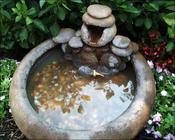
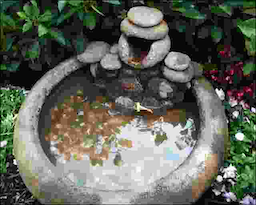
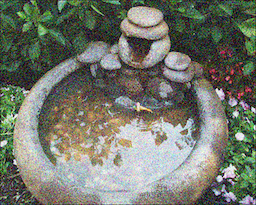
The most commonly encountered image distortions are White Noise (WN), Gaussian Blur (GB), JPEG compression, and JP2K compression. For example, the white noise distortion can be caused when taking pictures at night with a mobile, or the gaussian blur if not focusing correctly before taking the shot.

Literature Review

The image quality assessment (IQA) methods are mainly split into two categories (1) reference, and (2) reference-less or blind. A referenced algorithm requires a pristine (a reference that is considered to be good quality) and distorted images to calculate the quality score. Reference-based algorithms are widely used to measure how the quality is compromised after applying processes like image compression, image transmission, or image mosaic. For example, there is a trade-off with image compression; the higher the compression, the lower the perceived image quality. As another example, having an automated way to measure image quality helps companies to define the optimal compression parameters to maximize loading speed without compromising the user experience. On the other hand, blind methods are focused on processes where there is no access to pristine images. For example, in crowdsourced image acquisition processes, the distorted images are only available.

Initially, blind IQA algorithms were specific to distortion. Hence, to calculate the image quality score, it was required to determine the distortion type before the computation. So, two models were needed, (1) a model that predicts the distortion type, and (2) given the distortion type, a model that predicts the quality score. The overall performance of these methods was much lower, and the research efforts continued towards general-purpose methods.

Several researchers found that Natural Scene Statistics (NSS) and transformations like wavelet and Discrete Cosine Transform (DCT) domain are powerful discriminators to assess the magnitude of distortion in an image. These approaches dominated until they were replaced by new algorithms based on feature learning. Given enough data, these algorithms surpass the performance of those based on hand-crafted features. The main disadvantage is that the number of parameters explodes, increasing the risk of a lack of generalization.

Problem Statement

Image Quality Assessment (IQA) differs from other image applications. In contrast to classification, object detection or segmentation, IQA dataset gathering is based on complicated and time-consuming psychometric experiments (See CSIQ, TID2008, TID2013, LIVE IQA). Thus, the creation of large datasets is expensive as it requires the supervision of experts which are in charge of ensuring the correct execution of the methodology. Another limitation is that data augmentation cannot be used because the pixel structure of reference images must not be modified.

Methodologies

Most of the newest algorithms focus on feature learning. As previously stated, the main limitation of these methodologies is the necessity of extensive datasets to generalize. Nonetheless, the latest methods focus on hybrid approaches that as a first step, automatically learn quality-aware features and secondly an association of such features to a perceived quality score.

The objective of this section is to introduce three entirely different approaches that have achieved outstanding performance in comparison with previous methods. The first method is based on a deep neural network that is trained to learn an objective error map. The second method introduces the concept of multiple pseudo reference images (MPRI) and the extraction of features through high order statistics aggregation, and the third method leverages unsupervised k-means clustering to create an image quality characteristics codebook.

As mentioned previously, one of the significant challenges of Image Quality assessment is the cost of tagging images. However, Jongyoo Kim et al. [1], found a way to take advantage of large amounts of data by splitting the training into two steps (See Fig. 3):

Train a Convolutional Neural Network (CNN) that learns an objective error map.
Fine-tuning the CNN using the subjective scores.

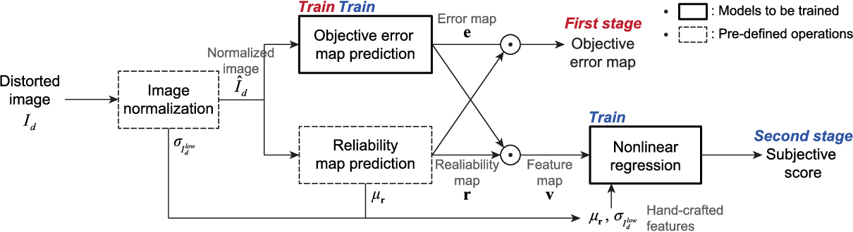
In the first step, there is no need to use human opinion scores because the CNN is trained to learn an error map between a pristine and a distorted image. We can extend the size of the first stage dataset using the concept of the pseudo reference image (PRI) and its distortion (See BMPRI algorithm below).

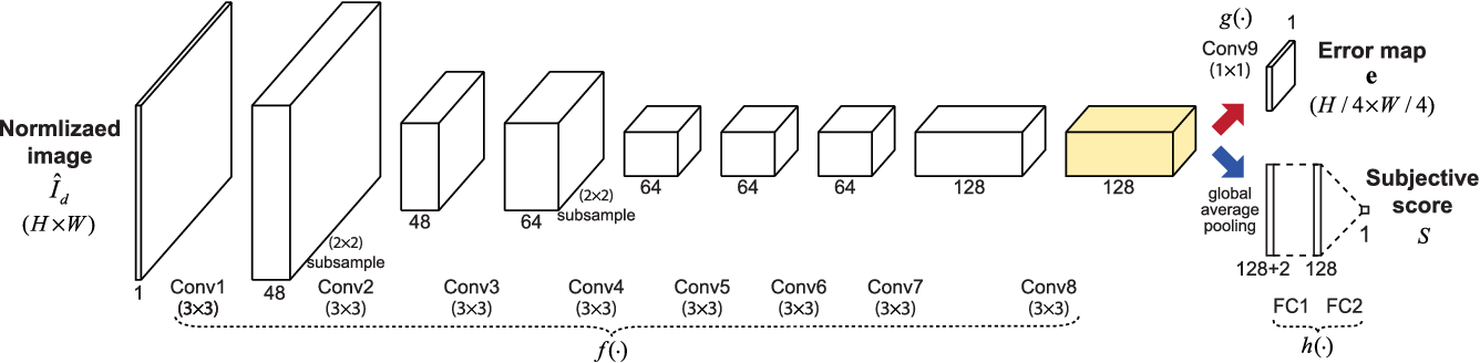
In the second step, two fully connected layers are added after the convolution 8 and fine-tuning is performed using the subjective scores to learn human opinions.

Learning Objective Error Map

The first stage is a regression with the objective to learn an objective error map. It is described by the red arrow in Fig. 4. The loss function is defined as the mean squared error of the predicted and ground-truth error maps. Moreover, the difference between such error maps is weighted by a reliability map prediction.

The reliability map prediction r has the function of avoiding to fail the prediction in homogeneous regions by measuring the texture strength of the distorted image.

The ground-truth error is just the difference between the reference image and the distorted image to the p power. The authors recommend a p=0.2 to have a broader error distribution from 0 to 1.

Learning Subjective Opinion

After the first model is trained to predict the objective error maps, a new network is created using the first network and adding two fully connected layers. In order to take advantage of images of different sizes, a global average pooling (GAP) is applied to the convolution 8 to turn it into a fully connected layer. The two handcrafted features μ and σ are concatenated to the FC1 (See Fig 4.) in order to compensate lost information. The loss function of this stage is defined as

where v is the global average pooling operation applied to the convolution 8.

The main idea of blind image quality estimation via distortion aggravation is to remove the concept of the reference image and use distorted images instead. Thus, the authors introduce the idea of multiple pseudo reference images (MPRIs). The MPRIs are generated from distorted images that are exposed to a severer amount of distortion. Therefore, pseudo reference image (PRI) generally has worse quality than its distorted equivalent.

The idea behind this methodology is to generate a series of PRI by further degrading the distorted image, and then measure the similarity between them using local binary patterns (LBP) to assess its quality.

Distortion Aggravation

According to the authors, selecting the distortion types is of utmost importance because different distortions introduce different artifacts, and it is needed to have consistent PRIs. For example, to estimate blurring artifacts, we can blur the distorted image. The selected distortions are JPEG, JP2K, gaussian blur (GB), and white noise (WN) to measure blocking, ringing, blurring, and noising artifacts.

where i∈ {1, 2, 3, 4, 5} indicates the i th level of distortion aggravation and k, and r, b, n indicate blocking, ringing, blurring, and noising effects.

Local Binary Patterns (LBP) Feature Extraction

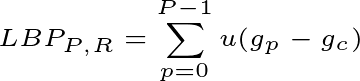
The LBP features are extracted for each of the MPRI and the distorted images. Originally, these features were used to classify different types of textures; therefore, allow us to detect structural changes.

where,

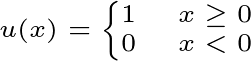
For simplicity, the authors recommend P = 4 and R = 1. For more details in extracting LBP features.

Similarities Between the Distorted Image and the MPRIs

To calculate the similarity between the aggravated image and the distortion, we define Lo as the overlap between the distorted image (Ld) and the MPRI (Lm) feature maps

where,

and then the quality is defined as.

Quality Prediction

After calculating the q score for all the previously defined aggravations, we need to concatenate all the resulting scores into a feature vector q that contains the descriptors of the distorted image’s blocking, ringing, blurring, and noising effects.

As the last step, a regressor is trained to map the feature vector q with the corresponding quality labels (MOS) of the images in the training set.

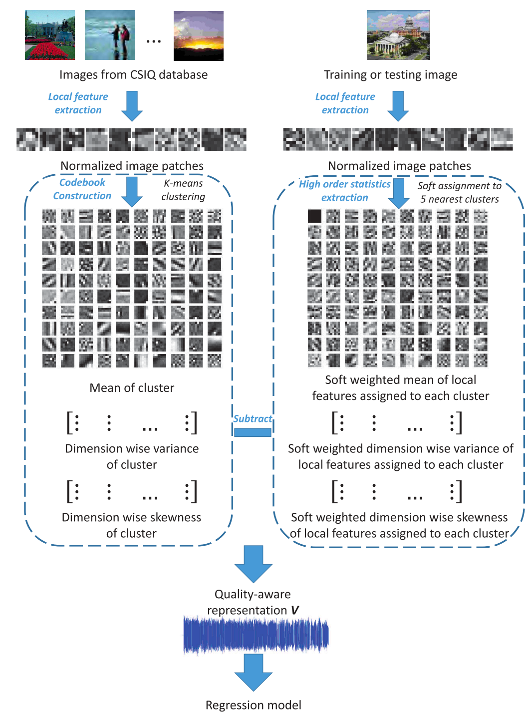
The HOSA methodology is a hybrid algorithm that takes advantage of an unsupervised learning stage that detects similar patches in a set of distorted images. This step is called codebook construction. Then, a second step uses a training dataset to find the similarities between each new patch and the five closest codewords in the codebook to train a regressor. This algorithm outperforms those based on hand-crafted features as it is more efficient in assessing images with text and artificial graphics.

HOSA algorithm is split into two different steps:

Codebook construction: A set of images is split into N patches which are used to create a codebook. The codebook is a set of K quality-aware codewords .
High order statistics aggregation: Given a new training dataset, for each new patch, the 5 nearest clusters are associated to be described with their high order statistics.

Local feature extraction

The overall idea of this method is to find a set of N normalized B x B image patches I(i, j) per image (local feature extraction phase). Each patch is normalized and then used to create a feature vector. This process is applied to all the pictures of the initial set. The authors picked the CSIQ database.

Codebook Construction

HOSA is not the only method that is based on a codebook. It is a framework followed by several authors to automatically detect image features that are useful to assess image quality. The codebook framework relies on the idea of splitting the image into informative regions. An informative area is called visual codeword, and a set of visual codewords form a visual codebook. The difference between the methods that are based on the codebook framework is the algorithm to create such codebook. In this methodology, the number of codewords is 100.

To create the codebook, given the set X comprised with local features of the initial dataset,K centers are found by minimizing the cumulative approximation error using K-means.

For each cluster, the mean, covariance, and coskewness are calculated.

High Order Statistics Aggregation

For each single local feature x in the training set,the r nearest codewords rNN(x) are selected by Euclidean distance. The authors recommend r=5. The residuals between the cluster mean and the r nearest codewords are calculated.

In reality, the soft weighted difference between the mean of cluster k and the mean of the assigned r local features for two different sets of features might generate the same m. Thus, the second, and third-order statistics are calculated for further discriminate different quality-level images.

Finally, for each local feature x in the training set, the first, second and third-order statistics are calculated for each cluster in the codebook and concatenated to create a single long quality-aware feature vector.

A regressor is trained to learn the subjective scores (i.e., mean opinion scores) using the quality-aware feature vector as the descriptor.

Performance Comparison

The Spearman rank-order correlation coefficient (SRCC) is used to compare the distinct methodologies. According to the results, the three methodologies perform similarly. They have in common the use of quality-aware learned features to calculate a score. In comparison to BRISQUE, a method that relies on hand-crafted features, there is a significant improvement in the SRCC.

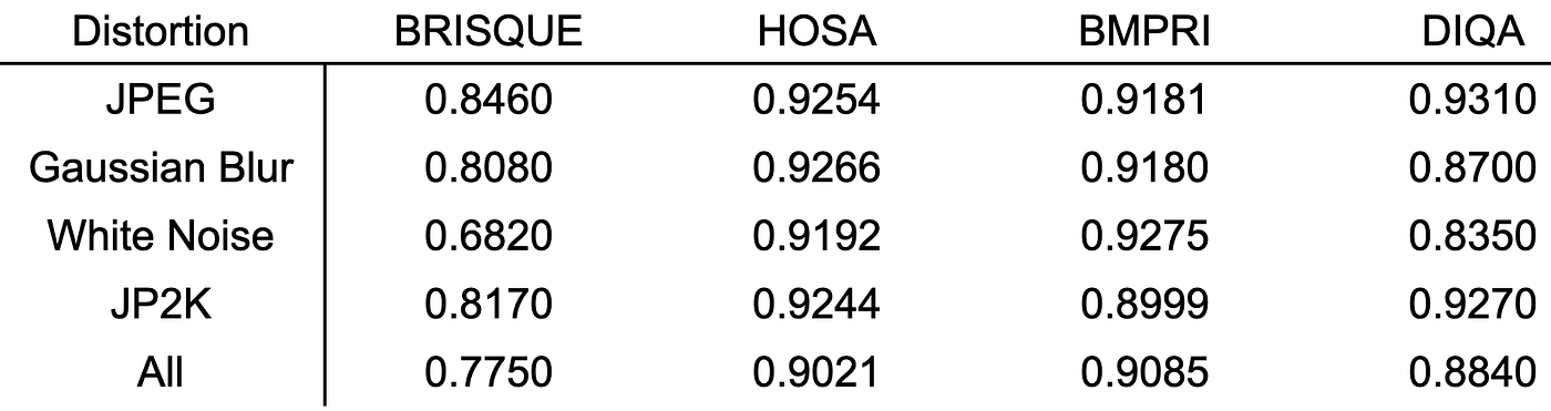
*Note: These results were gathered from each of the articles which might contain biased results. I am working on implementing each method to assess real results.

Jupyter Notebook

Implementation of DIQA with Python and TensorFlow 2.0

ocampor/image-quality

Conclusion

Three of the most recent methods for image quality assessment were briefly described. All of them are based on feature learning to detect distortions on images. According to the SRCC scores presented by the authors, these methodologies are consistently better than previous methodologies that rely on hand-crafted features to calculate image quality.

References

[1] Kim, J., Nguyen, A. D., & Lee, S. (2019). Deep CNN-Based Blind Image Quality Predictor. IEEE Transactions on Neural Networks and Learning Systems. https://doi.org/10.1109/TNNLS.2018.2829819

[2] Mezghani, LinaWilber, K., Hong, H., Piramuthu, R., Naaman, M., & Belongie, S. (2019). Understanding Image Quality and Trust in Peer-to-Peer Marketplaces. In 2019 IEEE Winter Conference on Applications of Computer Vision (WACV) (pp. 511–520). IEEE. https://doi.org/arXiv:1811.10648v1

[3] Min, X., Member, S., Gu, K., Zhai, G., & Liu, J. (2018). Blind Quality Assessment Based on Pseudo-Reference Image, 20(8), 2049–2062. https://doi.org/10.1109/TMM.2017.2788206

[4] Min, X., Zhai, G., Gu, K., Liu, Y., & Yang, X. (2018). Blind Image Quality Estimation via Distortion Aggravation. IEEE Transactions on Broadcasting, 64(2), 508–517. https://doi.org/10.1109/TBC.2018.2816783

[5] Xu, J., Ye, P., Li, Q., Du, H., Liu, Y., & Doermann, D. (2016). Blind Image Quality Assessment Based on High Order Statistics Aggregation. IEEE Transactions on Image Processing, 25(9), 4444–4457. Retrieved from https://ieeexplore.ieee.org/abstract/document/7501619/